Resources
 Part of the Oxford Instruments Group
Expand
Collapse
Part of the Oxford Instruments Group
Particle Imaging Velocimetry (PIV) is an optical method of flow visualization used in research and industry to obtain velocity measurements and related properties in fluids. This tech note details how to integrate the Andor Scientific CMOS (sCMOS) family of cameras, Neo and ZL41 Wave, into a PIV setup. (Note that the Neo cameras have been discontinued in June 2023)
The acquisition type described can be configured either in Andor Solis acquisition software or through use of the Andor Software Development Kit (SDK3). It is also possible to use 3rd party acquisition software environments such as LabView or MatLab. The Neo and ZL41 Wave both house a 5.5 megapixel sCMOS sensor, the unique architecture of the sensor presenting the only sCMOS device with both true global shutter and rolling shutter exposure modes, read noise down to 1 electron rms, dynamic range of up to 30,000:1 and full frame rates of up to 100 fps in rolling shutter, 50 fps in global shutter. The global shutter exposure mechanism will be utilized in a PIV double exposure configuration, offering an inter-frame time that is optically measured down to < 1 μs.
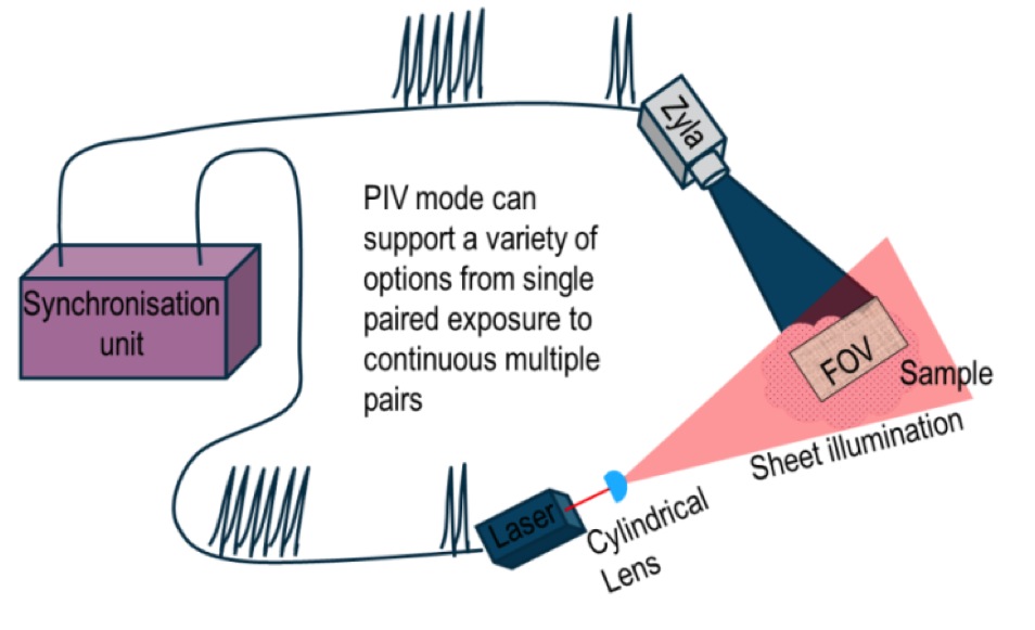
Figure 1: Typical PIV Setup
• The camera can be externally triggered and the length of exposure cycle controlled through the period of the input TTLs [External Exposure Trigger mode]
• The laser, or illuminating source, can be independently triggered.
• Sequences of images pairs are required having minimal temporal delay (down to sub-microsecond) between images within a pair.
Temporal resolution is a key parameter in this technique. A PIV set-up typically includes the following equipment:-
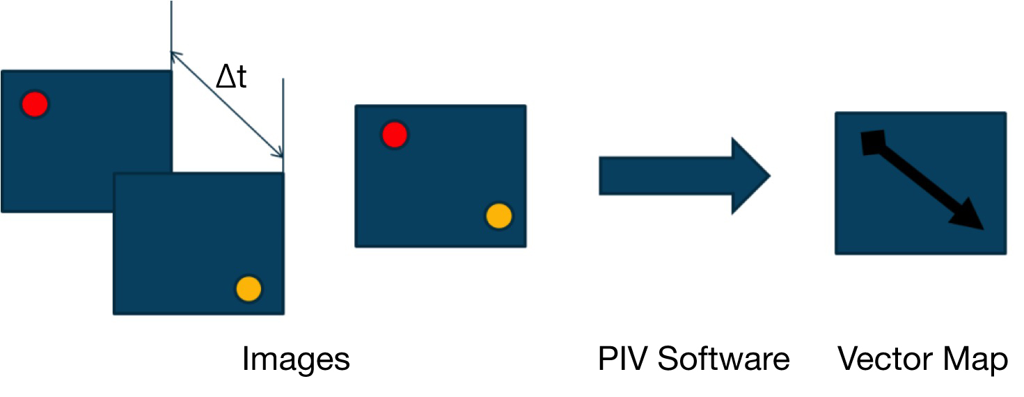
Figure 2: Image Processing
• Camera with lens
• Triggerable pulsed laser
• Cylindrical Lens
• Synchronization Unit
• PIV seed Particles
The laser’s beam is fantailed by a cylindrical lens to illuminate a plane of the sample which is imaged by the camera. The laser and camera are integrated using a device, such as the synchronization unit shown above, which will act as the master timing control unit.
The camera is configured to acquire a pair of exposures (although multiple exposure pairs can be configured) of the sample plane with minimal delay between the exposures. The length of the camera exposure is normally not a key requirement, with relatively long exposures commonly being used. The synchronization unit provides two pulses to the laser, or illuminating source, causing it to fire, once near the end of the exposure of the first image and then again at the beginning of the second exposure. The key timing parameter is the time Δt between the illumination pulses as this determines the temporal resolution for the two images, which are then processed to produce a suitable vector map derived from this time differential.
The technique usually requires some particles to be seeded into the medium in order to be observed. These particles enable the flow of the medium to be observed without altering the movement. These particles are illuminated, normally by a laser pulse or strobe, to enable their location to be imaged.
To use the ZL41 Wave or Neo sCMOS cameras for PIV we recommend the following camera settings:-
• Global Shutter
• External Exposure Triggering
• Overlap ON (meaning exposure to light while simultaneously reading out charge from previous exposure)
• 560 MHz readout speed (this is the maximum readout speed available)
• Kinetic sequence of 2 images or more (multiple of 2)
Note: other settings can be selected as required.
Figure 3 illustrates how the camera operates when combining Global shutter, External Exposure Trigger and Overlap readout mode, as recommended for PIV integration.
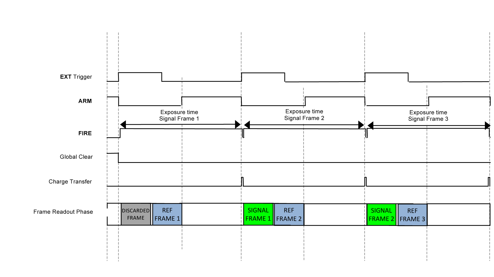
Figure 3: Timing diagram illustrating Global Shutter with External Exposure triggering
Global Shutter mode, which can also be thought of as a ‘snapshot’ exposure mode, means that all pixels of the array are exposed simultaneously. All pixels in the array are cleared of charge using the Global Clear before the exposure begins. At the start of the exposure each pixel simultaneously begins to collect charge and is allowed to do so for the duration of the exposure time. At the end of exposure, each pixel transfers the accumulated charge simultaneously to its read out node. Global Shutter requires a reference frame to be read out of the sensor in addition to the signal frame to generate a single image, therefore effectively halving the frame rate that would have been achieved in Rolling Shutter mode.
Combining Global Shutter with Overlap Mode means that a pair of camera exposures can be acquired ‘back to back’, separated only by the time to transfer charge into the readout node, referred to as the Charge Transfer time. This minimized gap between two subsequent exposures renders this configuration ideal for PIV operation.
The parameters shown in the Figure 3 are described as follows:
• FIRE: In Global Shutter mode, the FIRE output indicates the exposure period, which is identical for all pixels. This pulse is available to the user via the FIRE output pin.
NOTE: In Global Shutter Mode the behaviour of FIRE Row n, FIRE ALL and FIRE ANY are identical to that of FIRE and therefore not shown in the diagrams for clarity.
• ARM: The ARM output from the camera is used for external triggering mode to indicate when the camera is ready to accept another incoming trigger pulse.
• Global Clear: Global Shutter uses Global Clear to initiate the first exposure. When this pulse is HIGH, charge is drained from every pixel thus preventing the accumulation of charge on the sensor. When the pulse is LOW, any photo-electrons generated are accumulating within the pixels, ready for transfer to the sense nodes and subsequent readout. The falling edge indicates the start of an exposure.
• Charge Transfer: This signal indicates when charge in the pixel is transferred to the measurement node, effectively ending the exposure. The charge is transferred while the pulse is HIGH and is shown in the diagrams.
• Frame Read Out Phase: This signal indicates when reference and signal frames are read out of the sensor.
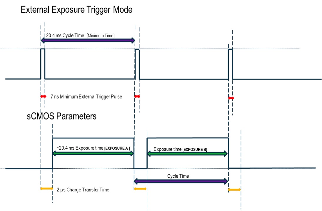
Figure 4: External Exposure Trigger Mode Timings for Neo, 560 MHz, full array, minimum exposure
In external triggering overlap mode, every positive edge of an external input TTL will trigger a Signal Frame read out and start a new exposure. The period of the external trigger pulse defines the cycle time. Note that when an acquisition sequence starts, the first positive edge of the trigger will initiate the first exposure, and internally the camera will perform a signal read and discard the frame. The subsequent positive trigger edge will end the first exposure, and initiate a new frame read out. The minimum exposure time is approximately the time to read out two frames. See synchronization section for further detail. If the period of the external trigger is less than the minimum exposure time some positive edges will be ignored.
In the timing diagram Figure 3, there is a small delay between the rising edge of the External Exposure Trigger and the actual start of the camera’s next exposure. This delay is due to the Charge Transfer time. The Charge Transfer Time for the specific readout speeds that are available in the Appendix, Table 2. Note that while the electronic signals indicate a charge transfer time of 2 μs at 560 MHz readout speed, when the time between 2 subsequent frames is measured by optical means, it is apparent the practical time between frames can be considered on the order of 100 - 250 ns. This is described in more detail later.
The timings can be estimated using the Tables 1 and 2 supplied in the Appendix. A more detailed timing scheme is illustrated in Figure 4, assuming a full 5.5MP frame readout at 560 MHz readout speed; faster frame rate speeds can be achieved if a smaller ROI is selected. As mentioned, the period of this trigger defines the cycle time. The first rising edge triggers the start of the exposure, and the subsequent trigger, assuming it has occurred after the minimum exposure time, ends the exposure and starts the next exposure cycle. The relationship between the exposure and the external trigger is shown in the schematic. Please note, it is important that both start and end triggers are available to complete the required exposures.
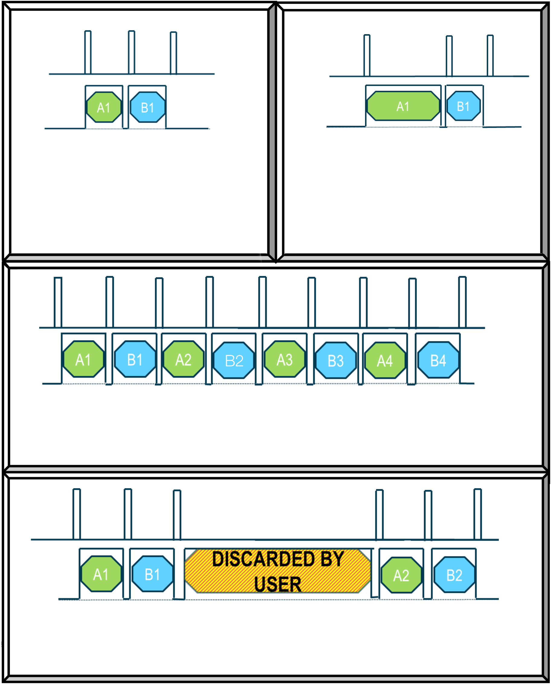
Figure 5a (top-left): Classic PIV Mode, Single Pair. This is the most basic setup, two images taken back to back with minimum delay between exposures.
Figure 5b (top-right): Classic PIV Mode, Single Pair with different exposures. The exposure time is controlled by the external exposure so it is possible to have images of different exposure length taken back to back
Figure 5c (center): Long sequence of paired PIV images. The images do not need to be single pairs but can be setup in long sequences. The exposure time can be varied image to image if required.
Figure 5d (bottom): Paired sequence with long delays between paired images. In this case a set of images is required with a long delay between their capture. This would require an extra exposure to be taken and the image discarded by the user.
As can be seen in Figure 4, the external exposure trigger initiates the exposure cycle. This commences with the Charge Transfer Pulse then the exposure begins, please note the exact duration of the exposure time is therefore the period of the external exposure trigger minus the charge transfer time. Once the second external exposure trigger arrives, the present exposure is terminated and the next exposure cycle begins.
The ARM output from the cameras can prove very useful when optimizing PIV synchronization. ARM indicates when the camera is ready to accept a new trigger and it only goes high when the camera has finished the processing of two frames. These two frames consists of the signal frame from the previous exposure (if this is the first exposure this signal frame is discarded) and the reference frame from the present exposure, as shown in the timing diagram in Figure 3. This defines the minimum exposure that can be readout.
External exposure triggering allows for a wide variety of sequences to be easily setup, allowing the user to select their own optimal mode of operation. The diagrams below show a selection of external trigger sequences in which the camera can be configured to capture images. In the individual diagrams the top trace represents the external trigger pulses, shown relative to the individual acquired images in the bottom trace. The images are identified with ‘A’ or ’B’ and a number, to indicate their position within the pair and the sequence. This is only a selection of example setups and is far from complete; other combinations can also be used but are not shown here.
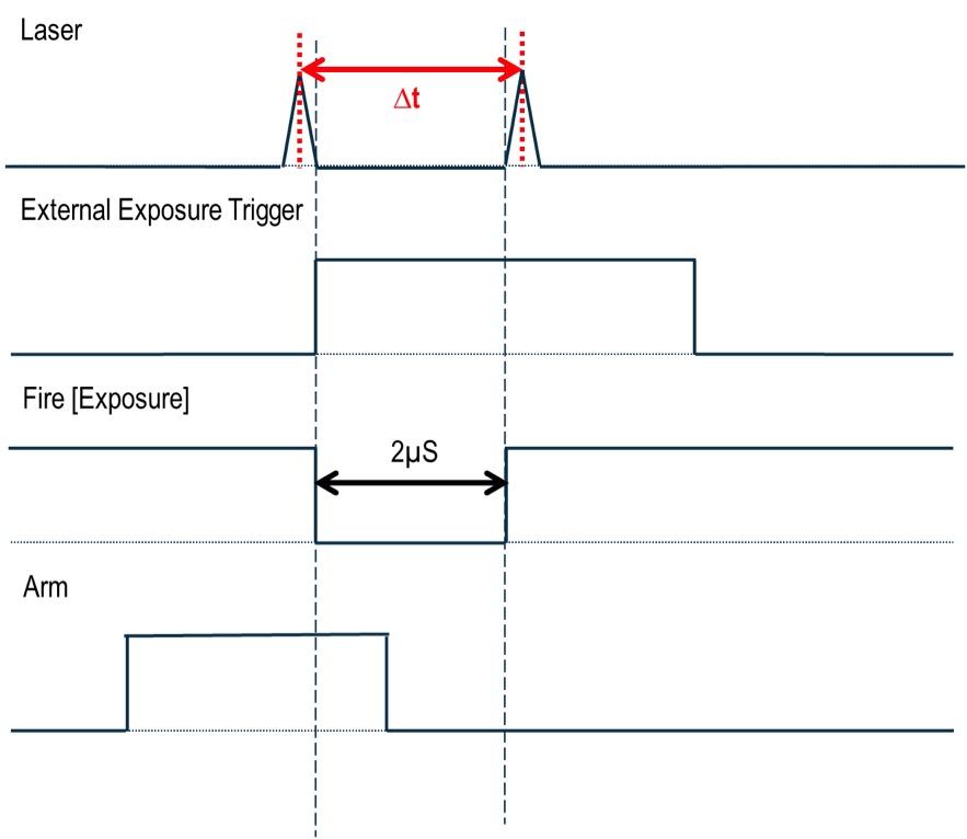
Figure 6: Optimal Inter-Exposure Timings
As it is desirable in PIV applications to minimize the time separation between the successive illuminating laser pulses, it is standard to trigger a laser pulse at the end of the first exposure and then again at the beginning of the second exposure.
The timing diagram, Figure 6, details the timing relationship between the laser pulse and the camera.
The key camera elements to achieving synchronization are the period of the External Exposure Trigger, the Arm and the minimum achievable exposure. Note, the second laser pulse can be moved relative to the first, thus altering the time delay between successive pulses.
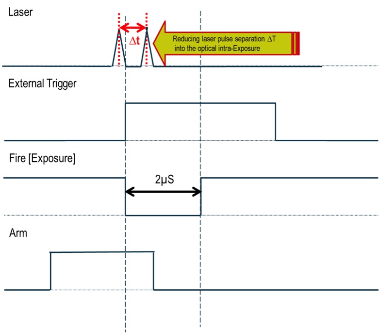
Figure 8: Optimal Optical Inter Exposure Timings
The relative timings shown in Figure 6 relate to the electronic signals of the camera; however the optical response of the sCMOS structure permits a smaller inter-exposure delay to be achieved. The diagram below shows the results of scanning a discrete laser pulse across the inter-exposure gap. The frames relate to the end and start of new exposures.
While the electronic signals indicate a charge transfer time of 2 μs at 560 MHz readout speed, when the time between 2 subsequent exposures is measured optically it is apparent that the time between the images can potentially be on the order of hundreds of nanosecond timing regime, if the system is optimally timed. In fact, recent evaluation of the ZL41 Wave camera by an experienced PIV customer concluded that an inter-frame gap of 100 ns could be readily employed.
However, it is advised that such a timing profile is individually mapped by the user within their system, to achieve the optimal regime for the laser pulse relative to the camera readout.
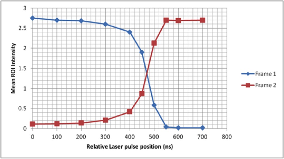
Figure 7: Mapped Inter-Exposure delay, note this graph is for indication only
1. Recommended Software Versions for PIV acquisition
The enhanced camera timings features which augment a PIV mode of operation have been added to the Andor Software as detailed below. Please note if an earlier version is used than stated below, there will be a jitter between every inter-exposure period amounting to approximately 1 row readout (10 μs).
| Camera Trigger | Trigger Jitter | Software Version |
| ZL41 Wave and Neo | Start Only | Solis 4.22 + SDK3 3.5 or later |
Table 1: Software Version with PIV Mode
2. Timing Tables for FULL Sensor Array
| Parameter | 560MHz | |
| Neo | ZL41 Wave | |
| Inter-frame | 84.3 μs | 83.2 μs |
| Charge Transfer Time [CTT] | 2 μs | 2 μs |
| Row | 9.37 μs | 9.24 μs |
| Frame | 10.1 ms | 9.98 ms |
| Clock Cycle | 3.57 ns | 3.52 ns |
Table 2: Software Version with PIV Mode
| Parameter | Timing Functions | Sensor Readout Speed 560 MHz |
||
| minimum | maximum | Neo | ZL41 Wave | |
| Exposure Minimum [Ext Trig period] | 2 frames + 2 interframes | 20.4 ms | 20.13 ms | |
| Cycle Time [Ext Trig period] | 2 frames + 2 interframes + CTT | 20.4 ms | 20.13 ms | |
| Acquisition Start Delay | 1 row | 9.37 μs | 9.24 μs | |
| Ext Trigger Pulse Width | 2 sensor speed clock cycles | 7 ns | 7 ns | |
| Fire Low Period | 20 sensor speed clock cycles | 71 ns | 70 ns | |
| Trigger Jitter | 1 row | 9.37 μs | 9.34 μs | |
Table 3: The timing functions, using the unit timings, with the actual timings for the parameter for the available readout speeds
Explore our related assets below...
© Oxford Instruments 2024