Confocal Raman microscopy is a non-destructive imaging technique for comprehensive analyses of organic polymer
composition, distribution, and defects. This tutorial presents a complete step-by-step workflow for performing initial
Raman measurements on polymer samples. It includes practical tips for choosing the region of interest (ROI), selecting
the measurement type, and setting key acquisition parameters. It also covers essential data evaluation steps. By
following this workflow, you can create high-resolution chemical maps of polymer samples, and extract Raman spectra of
individual components with confidence.
All steps described can be carried out using Oxford Instruments’ witec360 Raman microscope equipped with the
Hexalight spectrometer, providing high resolution, speed, and sensitivity.
Step 1: Defining measurement goals for Raman imaging of polymer samples
The first step in a typical polymer measurement workflow is to define the goal of the experiment. Examples include:
- Identifying which polymers the sample contains
- Determining how different polymers are distributed within the sample
- Studying defects in the polymer
- Detecting contaminations
- Investigating polymer aging
Step 2: Preparing polymer samples for Raman measurements
Generally, minimal sample preparation is required for analysing polymers with Raman. Most polymer samples can be
placed directly onto the microscope stage, or a small section can be cut out for investigation. Ensure the sample is
mounted securely to prevent drift.
Depending on the measurement objective, additional preparation might involve cutting a representative piece of the
polymer and fixing it on a sample holder. For investigation of the sample composition and distribution of the
components, a piece large enough to contain all components, but small enough to fit easily into the microscope is
ideal. A piece between a few mm2 and a few cm2 is usually sufficient. When studying defects or
contaminations, the sample should include at least one.
Step 3: Setting up Raman measurement parameters for polymer analysis
Begin the polymer analysis by obtaining an overview image using the video mode of the Oxford
Instruments witec360 Raman microscope. Depending on the microscope configuration, select from white-light illumination
modes such as reflection, transmission, or darkfield. If multiple options are available, choose the mode that best
highlights the ROI in the sample. A fast overview of the sample is gained with low magnification objectives like 5x or
10x. Then, use a high magnification objective like 50x or 100x for detailed imaging of the desired area (Figure 1).
Define the region to be analysed with Raman using this image.
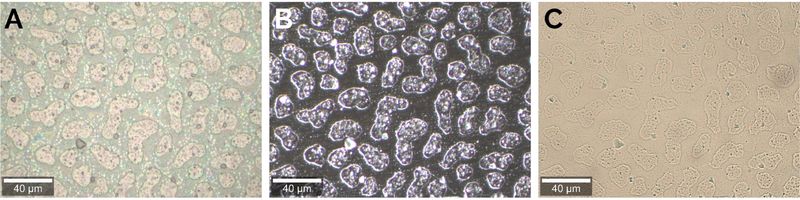
Figure 1: Examples of video images of a copolymer sample in different modes, recorded with a 50x objective: (A)
reflection, (B) darkfield, (C) transmission mode.
Before starting the Raman measurement, adjust parameters in “Oscilloscope Mode”, i.e. using the live
spectrum from the sample. To maximise Raman signal and spatial resolution, use an objective with the highest possible
numerical aperture, for example 100x/0.9.
Start with a 532 nm (green) laser, which typically generates strong Raman signals. If the sample
burns, melts, or exhibits strong fluorescence under 532 nm, switch to an alternative wavelength. Note that shorter
wavelengths produce higher Raman signals and better spatial resolution, but increase the risk of sample damage.
Set the laser power to the highest value that does not damage the sample while maximising signal (as
high as possible but as low as necessary).
Then adjust the integration time to optimise the balance between acquisition speed and
signal-to-noise ratio (S/N). Avoid detector saturation to prevent non-linear effects.
After all parameters are defined, record several single Raman spectra from different positions to
gain an initial understanding of the sample composition. Set the integration time as described for the “Oscilloscope
Mode”, and apply ~5–20 accumulations to get Raman spectra with high S/N ratio.
For another quick evaluation, perform a “Line Scan” in any chosen direction. This reveals
transitions between different sample components, or determines sample thickness and/or transparency (“Line Scan” along
Z axis).
Finally, Raman imaging in the XY plane (area) or XZ plane (depth) reveals sample heterogeneity, the
distribution of different components, contaminations, or defects. “Depth” scans show the layers in the sample, while
3D scans (image “stacks”) visualise the 3D distribution of different components. Adjust the pixel size for the Raman
image depending on the desired spatial resolution and the size of the relevant sample features. Large-area,
high-resolution Raman images may require overnight acquisition. The software estimates the measurement duration,
allowing parameter optimisation also with respect to the available time.
All generated objects (e.g. video images, single Raman spectra, Raman images, and processed data) appear in the
Project Manager and are stored together in one project file. This can be opened in the data evaluation software
(PROJECT), and the data can easily be processed while a new measurement is running.
Step 4: Analysing Raman microscopy data and polymer composition
The first steps in Raman data analysis are cosmic ray removal (CRR) and background
subtraction. The PROJECT software provides a guided workflow (wizard) through these steps. Several
algorithms and preview options facilitate the correct selection of parameters for both operations to preserve the
Raman peaks (Figure 2A, B).
Smoothing of the Raman spectra increases S/N ratio, but can distort Raman peaks (Figure 2C). Apply
it only when other ways of improving S/N (e.g. increasing laser power or accumulation time) are not feasible.
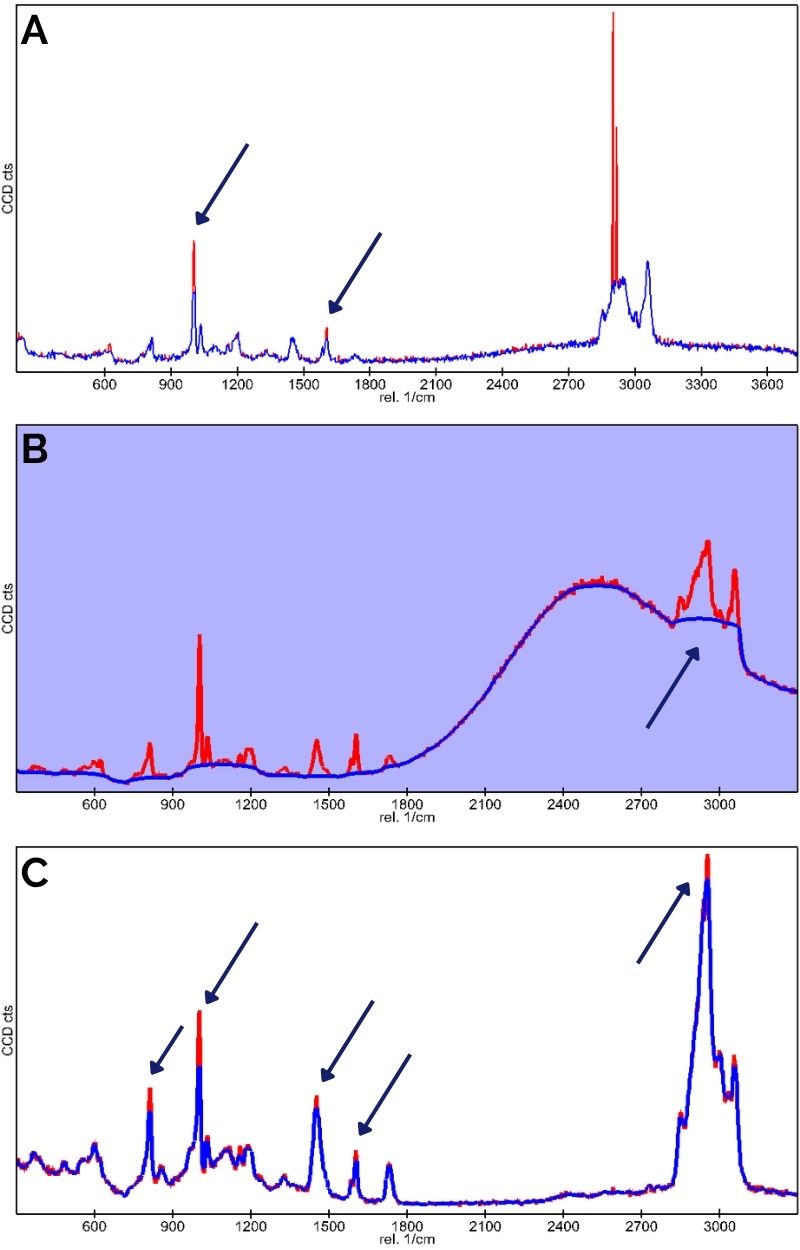
Figure 2: Examples of excessive processing of the polymer Raman spectra. Arrows indicate where the Raman signals are
significantly altered: (A) excessive CRR; (B) excessive background subtraction; (C) excessive smoothing.
For heterogeneous samples, use TrueComponent analysis to find all components in a Raman image.
Component identification may be manual (assisted by the software) or fully automatic. Average all spectra of identical
components to improve the S/N ratio.
For Raman spectra representing a mixture of several different chemicals, apply the demixing function
to obtain pure spectra (Figure 3). Ensure that no part of any Raman spectrum becomes negative during demixing.
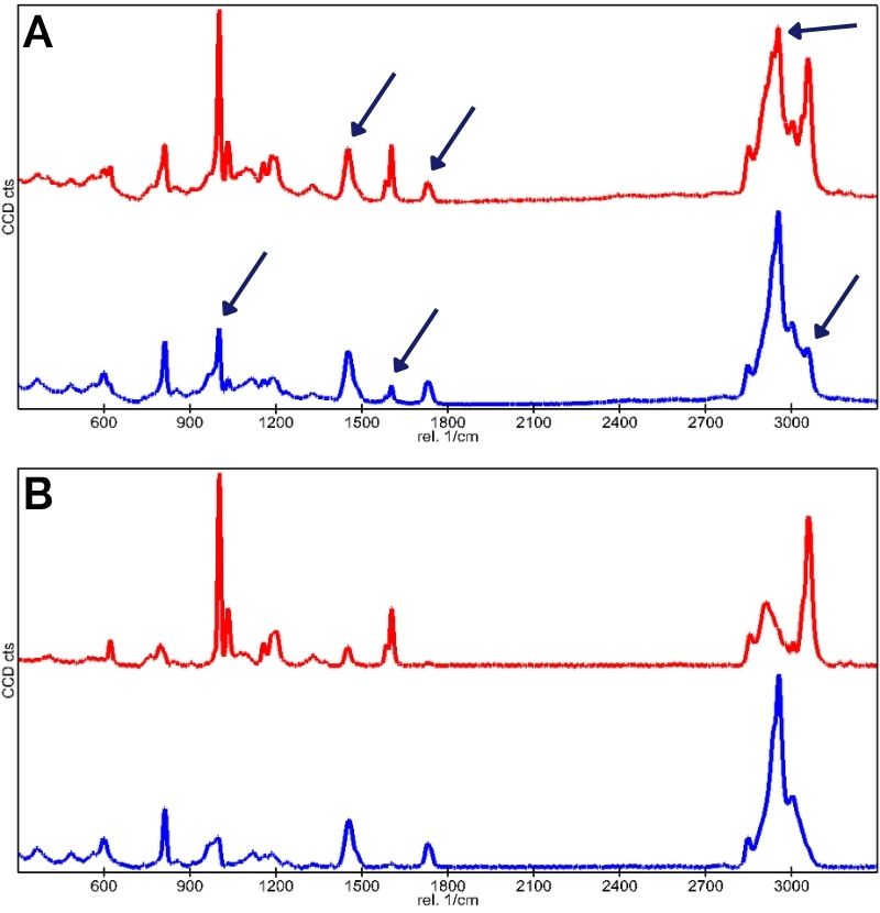
Figure 3: Example of Raman spectra demixing: (A) Raman spectra before demixing; (B) Raman spectra after demixing.
Identification of unknown sample components can be performed with TrueMatch using
commercial, free, or custom-built spectral databases.
After the analysis, the obtained Raman image visualises the spatial distribution of the identified
chemical components, revealing sample heterogeneity, composition, contaminations, and defects. In the presented
example, the two polymers polystyrene (PS) and poly(methyl methacrylate) (PMMA) were identified by their Raman
spectra, and their spatial distribution was visualised in a Raman image of the blend (Figure 4).
The full analysis presented in this tutorial can be done in less than a minute using the PROJECT software’s guided
data processing.
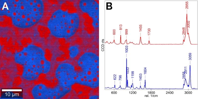
Figure 4: High-resolution Raman image of a copolymer sample after data processing: (A) Raman image colour-coded
according to the identified polymer components PMMA (red) and PS (blue), (B) corresponding Raman spectra with the same
colour code.
Summary: Key best practices for Raman imaging of polymers
Raman imaging is a reliable, non-destructive method for chemical analysis of polymer composition, distribution,
defects, and contamination. This guide presents a workflow for performing accurate, high-quality Raman measurements of
polymer samples: from defining measurement goals through sample preparation to data acquisition and analysis. Oxford
Instruments’ advanced Raman systems are designed to simplify workflows, improve accuracy, and save time.