Introduction
The AutoPhaseMap module in the Oxford Instruments' EDS software, AZtecEnergy, automatically finds areas of different characteristic composition from X-ray map data, and determines the distribution, area, constituent elements and composition of each of these areas or phases. This application note examines how this technique can be used to determine and characterise the phases present in an igneous rock. Finally the results obtained are compared to the phase mapping results calculated from an EBSD dataset collected simultaneously with the EDS acquisition, to validate the result of the AutoPhaseMap method.
Automatic Phase Mapping and Phase Identification
The sample analysed was from an oceanic gabbro. The sample analysed was polished but uncoated and data was collected at a high tilt to allow simultaneous EBSD data collection. A variable vacuum was used to reduce charging effects. An X-ray SmartMap was collected from an area of the sample under the conditions shown in Table 1 below.
| Accelerating Voltage (kV) | 20 |
| Sample tilt (°) | 70 |
| Map resolution | 259 x 228 |
| No of pixels | 59052 |
| Counts per pixel | 163 |
| Chamber pressure (Pa) | 20 |
Table 1. Acquisition parameters for SmartMap Acquisition.
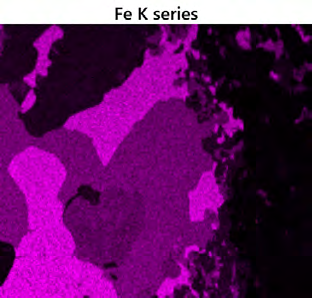
X-ray maps for the major elements identified in the sample are shown in Fig. 1. These maps provide detailed information about the distribution of elements within the sample, and can be used to deduce the phase and chemical composition of the sample by reconstructing spectra from representative areas and interpreting the constituent elements and quantitative results from this data.
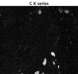
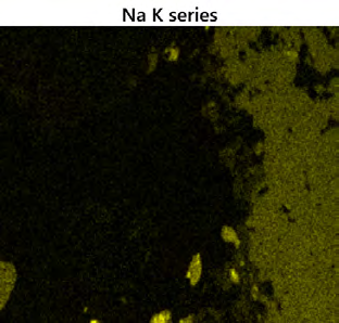
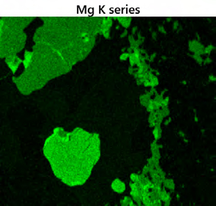
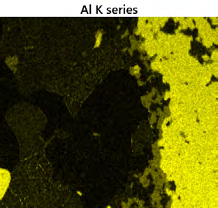
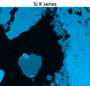
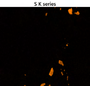
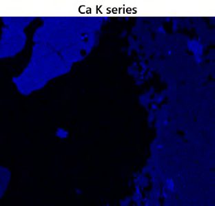
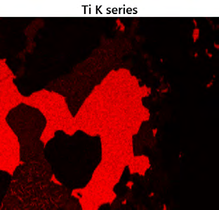
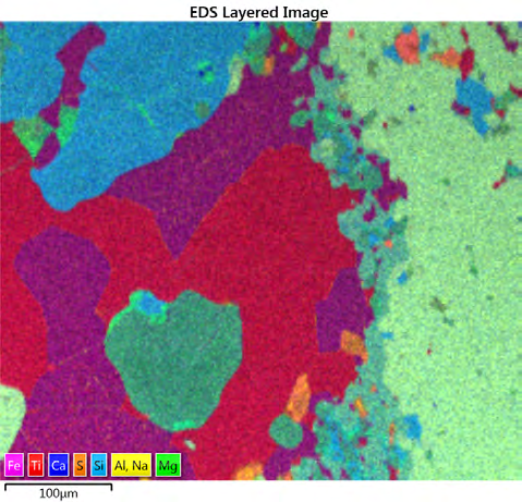
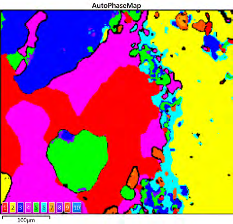
One powerful method to make the visualisation of the sample easier, is to overlay the X-ray maps in order to make a single coloured "Layered Image" of the sample (Fig. 2a). Using this image, the overall phase distribution and micro-structure of the sample is shown. From the X-ray mapping information, AutoPhaseMap will calculate areas of characteristic chemistry and determine their spectrum, composition and distribution in just a few seconds. These areas of different chemistry will correspond closely to the different phases in the sample. The calculated AutoPhaseMap is shown in Fig. 2b. The colour assigned to each phase is determined by the hue in the Layered Image, so that the result can be more easily related to the colours and intensities of the X-ray maps. Each phase is given a number shown in the colour key of the AutoPhaseMap and this corresponds to the phase number in the Phase Details table (Fig. 2c). This table also gives the area fraction of the identified phase. By default, the AutoPhaseMap software gives each phase a name: this consists of the major elements in the phase, with cations given first. The phase names can easily be modified and, in this case, mineral names have been assigned to each phase based on inspection of the spectra and composition of each phase.
(a)
(b)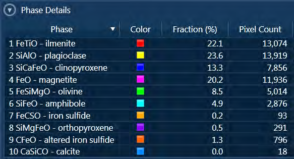
(c)
Fig. 2. a) Layered image where X-ray maps for Fe (magenta), Ti (red), Ca (blue), S (orange), Si (light blue), Al and Na (both yellow) and Mg (green) have been overlayed. b) AutoPhaseMap composite image showing the distribution of the identified phases. c) Phase details table showing the phases identified and the area fraction of each phase.
In addition, the AutoPhaseMap software displays (for each phase): a phase image showing the distribution of the phase, a spectrum calculated by summing the pixels identified as belonging to that phase and a quantitative result for each phase giving the average phase composition. The results for phases identified in the oceanic gabbro are shown in Fig. 3.
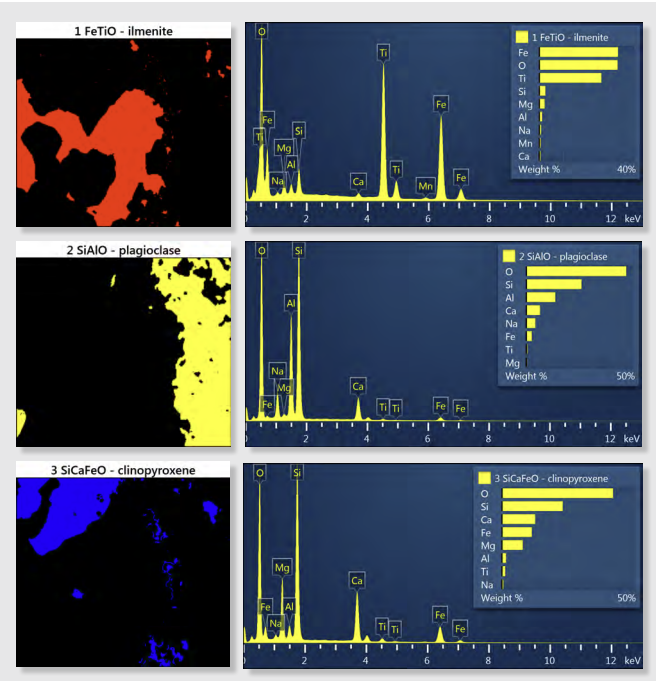
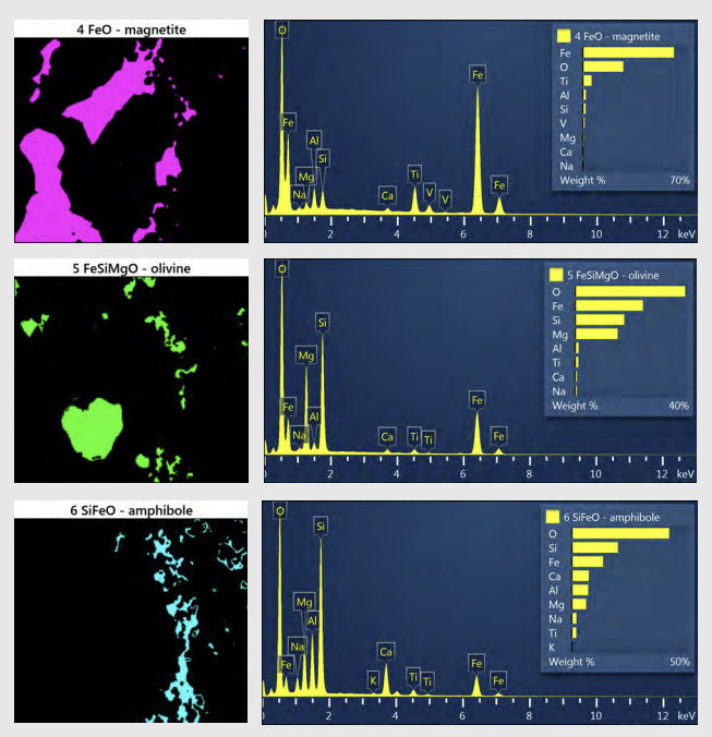
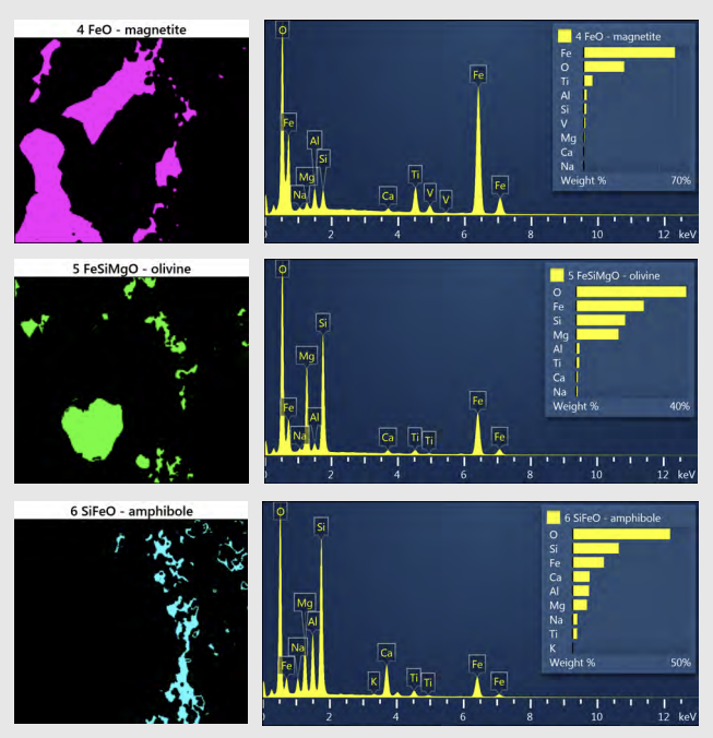
Fig. 3 (1-10). AutoPhaseMap results for the ten phases identified in the oceanic gabbro sample.
Discussion
AutoPhaseMap found six major phases: four silicates (plagioclase, clinopyroxene, olivine and amphibole) and two oxides (magnetite and ilmenite). Due to the beam skirting caused by the variable vacuum, some cross-talk of the constituent elements is seen - for example with Al, Na and Ti. Reasonable compositions for the minerals are also seen, despite the high tilt angle of the sample and the variable vacuum.
A significant number of minor phases were found by the software. One further silicate, 8 MgFeSiO, is similar to olivine, but has four cations calculated to 6 oxygens consistent with orthopyroxene, commonly found with clinopyroxene in gabbros. A significant number of phases were also identified with Fe and S with varying amounts of carbon, oxygen and sodium. This probably represents an iron sulphide that has reacted later and altered to other phases. The original iron sulphide may be represented by 7 FeCSO, which has a Fe/S ratio of about one suggesting pyrrhotite (Fe1-xS) rather than pyrite (FeS2). The other phases have been merged together manually to form Phase 9 CFeO, which surrounds the grain of iron sulfide and is also found together in other similar sized grains in the sample, which coincide with high carbon intensities seen in the carbon X-ray map (Fig. 1). AutoPhaseMap also found two very small areas of a different carbon containing phase 10 CaSiCO; these are very small and probably have a significant cross-talk contribution from nearby clinopyroxene and olivine. If additional contributions for the elements of these nearby minerals are taken into account, the main constituent elements for this phase are carbon, oxygen, calcium suggesting a carbonate such as calcite, presumably the result of post formation chemical processes perhaps associated to those that altered the iron sulfide.
Validation of the AutoPhaseMap Result with EBSD
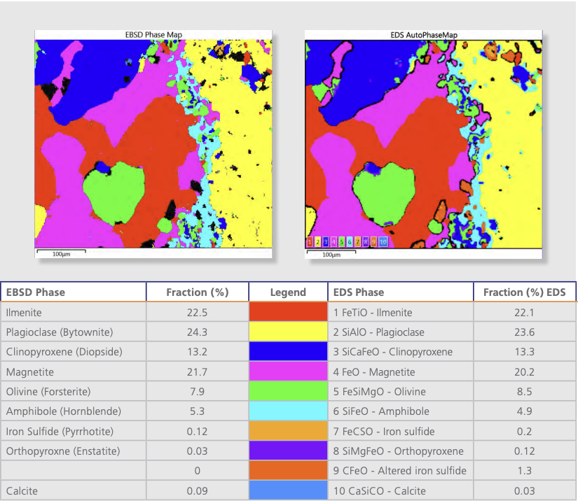
EBSD mapping is a more established method for phase analysis, analysing the backscattered electron diffraction pattern produced at each pixel location to discriminate the correct phase among a set of possible crystal structures. In this way it identifies phases much more directly than the EDS-based characteristic chemistry AutoPhaseMap method. The phase maps generated by the two techniques are compared in Fig. 4. EBSD phase colours were chosen to colour phases similarly with their counterparts in the AutoPhaseMap for easier comparison. On first sight, the similarity of the results is encouraging and validates the AutoPhaseMap result obtained. On closer inspection, differences reveal the different strengths of the two methods. A strength of the AutoPhaseMap method is its relative insensitivity to surface preparation, unlike EBSD: for example phases/areas which do not give patterns still have characteristic chemistry. Thus black areas in the EBSD map, which yielded no patterns, are shown to be mainly areas where altered orthopyroxene, olivine, and various states of alteration of iron sulfide have been found by EDS. EBSD is particularly useful in confirming more precisely phase identification. For example, in the region identified by EDS as being most likely to be an iron sulphide (7 FeCSO - light orange), the EBSD result not only confirms this - but also that the mineral is pyrrhotite (Fe1-xS) rather than pyrite (FeS2). It can also been seen in other areas that the much higher spatial resolution of the EBSD technique at 20kV yields more precise results on finer scale structures and grains. For example, in the area where EDS finds a possible calcium carbonate and EBSD confirms it to be calcite, and in some of the areas where smaller grains of olivine (green) and clinopyroxene (blue) are found together. Collecting the data at higher resolution would probably improve the results of the EBSD and particularly the EDS in this respect.
Conclusion
AutoPhaseMap finds the main phases present in the sample, and also provides some more detailed information where one of the minerals, pyrrhotite, has reacted and broken down. It provides information about phase distribution, constituent elements and composition. It provides in seconds an extra dimension of information on top of X-ray mapping data that can be used to understand the history of generation and alteration of a sample. EBSD has been used to validate the AutoPhaseMap result and shows similar results which differ only in fine detail due to the different strengths of the two techniques.
Acknowledgement:
Dr. P. Trimby of The University of Sydney provided the oceanic gabbro sample for this study.