Application Notes
Imaging Rock Cores with NMR/MRI
Published: 03 Nov 2026 · Last updated: 03 Nov 2026
This Application Note was created in collaboration with Green Imaging Technologies

Introduction
The main advantage of utilizing NMR or MRI technologies to investigate rock cores is the ability to study the fluid within the pore network. Using imaging applications, we can directly measure the fluid content as a function of position (spatially resolved imaging). In addition, nuclear magnetic resonance (NMR) properties such as pore size distributions (T2) can be spatially resolved highlighting information about the fluid or the environment of the fluid as a function of position in the sample.
In the past, hardware limitations made imaging measurements time consuming to the point of making them impractical for many users. Current hardware and data acquisition methods have largely overcome this limitation and made NMR/MRI imaging applications more accessible to a wider range of users.
Users also have access to NMR compatible overburden, or pressure, cells which allow for the imaging of fluids under pressure, flowing through the pore network in a rock core. Both two dimensional and three-dimensional images of these flow experiments can be obtained.
Fluid Distribution
NMR/MRI imaging techniques provide one of the best methods for examining the distribution of hydrocarbons or other fluids in a rock core. Using various saturation and flooding methods, many different phenomena can be explored with NMR/MRI technology. Fluid fingering, pore connectivity and fluid typing experiments can all be used to create an accurate picture of what is happening with fluids within the rock core samples.
Porosity is a common parameter measured using NMR, typically resulting in a distribution of pore sizes. NMR imaging can take this a step further to provide information on the heterogeneity of porosity throughout the rock sample. Figure 1 shows the result of such a measurement, utilizing a two-dimensional fast spin echo (FSE) experiment showing the location of the brine in a brine saturated limestone rock.
The higher signal intensity indicates areas of higher porosity in the rock. This sample is very heterogeneous with large variations in porosity throughout the rock.
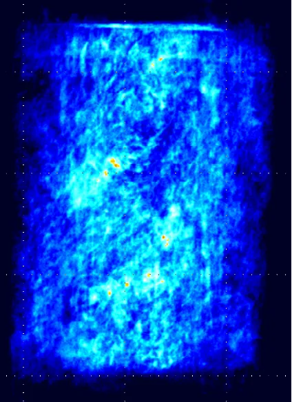
Fig. 1 — 2D FSE 512x512 (resolution of 0.117mm), 16 shots, 64 signal averages, scan time of 43 minutes. High intensity indicates large pore heterogeneity distributed through the 1½" sample.
Employing image processing (windowing and leveling the image), the connectivity of the pores can be examined. Figure 2 shows a three-dimensional FSE image showing the connection of the larger pores.
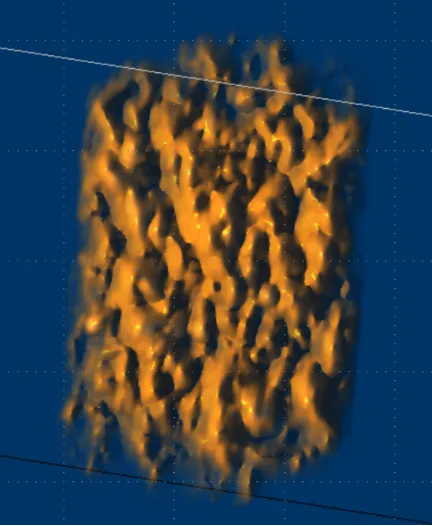
Fig. 2 — 3D FSE 128x128x128, 16 shots, 16 signal averages, scan time 9 minutes. Windowed and levelled to show only the high intensity porosity which indicates large pore heterogeneity distributed through the 1½" sample.
The NMR properties of the fluid in the rock help determine which imaging technique is best suited to the samples under study. For example, FSE requires the T2 to be long enough to have signal at the later echoes. A typical FSE sequence uses an echo time of 2–3 msec so if 16 echoes are encoded in each shot then the T2 should be longer than 30–40 msec. The table at the end of this document provides a quick reference for determining what pulse sequence should be used.
Spatially Resolved NMR Properties
NMR properties such as T1 and T2 can be spatially resolved to investigate differences within the rock. These differences can be anything that is known to affect the NMR properties such as pore size, fluid saturation (brine or oil), and wettability.
Figures 3 and 4 show an image of a limestone sample fully saturated with brine. Each two-dimensional pixel contains a T2 distribution. One way to visualize the data is to produce an image which contains only a single T2 value. With the intensity scale fixed, it can easily be seen how much each T2 (which represents the size of the pore) is contributing to the total porosity.
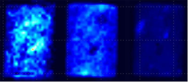
Fig. 3 — 2D 48x48 4 NSA Scan Time 16 hours. Each plot shows the image of fluid with a specific T2 value. Left is a long T2, middle an intermediate T2 and right a short T2 value. All images are shown on the same intensity scale.
If each image is scaled independently, the location within the rock of the small and large pores can be determined.
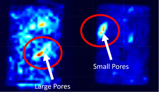
Fig. 4 — 2D 48x48 4 NSA Scan Time 16 hours. Left plot shows an image of only the large pores (long T2s) and the right shows only the small pores (short T2 components). Each image is individually scaled. You can easily see clusters of large and small pores.
Enhanced Oil Recovery – Wetting Properties
NMR and MRI are excellent tools for evaluating enhanced oil recovery (EOR) and investigating wetting properties of the rock sample through imbibition studies. Understanding the wettability of a reservoir is key to determining the effectiveness of EOR strategies.
A dry rock sample can be placed in a small 1–2 mm layer of brine to observe the imbibition process as the brine is pulled up through the rock. This process will be governed by the capillary forces and wetting properties of the rock.
Figure 5 shows a time series of 2D FSE images where the rock is allowed to imbibe brine from the bottom of the rock.
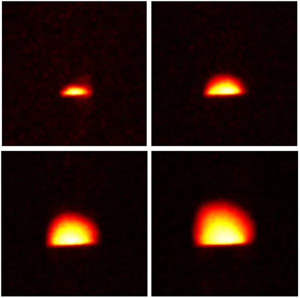
Fig. 5 — Time series of 2D 64x64 FSE images. Each image is acquired in 35 seconds.
Following the imbibition of approximately 20 minutes, a series of images was acquired (Figure 6) to visualize the redistribution of fluid through the rock. These images were taken over the course of two hours.
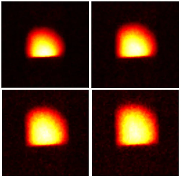
Fig. 6 — 2D 64x64 FSE images taken during the redistribution of fluid (2 hours).
These 2D images provide a visualization of the fluid redistribution in the rock core, but NMR can also provide a range of other useful information from these images. The capillary forces at play can be derived from these images, as well as information about the connectivity of the pore network and the permeability of the reservoir in question.
Which Acquisition Should I Use?
GeoSpec NMR instruments with GIT Systems software provide several pulse sequence options for acquiring 2D and 3D images of rock core samples. Several parameters are taken into account to decide which technique is best suited to the rock samples being measured. The table below provides a quick reference guide to the different techniques and when to use each one.
| Technique | T2 | T2* | T1 |
| FSE | Long > Tau * 2 * number of echoes | Long > resolution / 2 / filter bandwidth | Long — due to T1 > T2 |
| SE-SPI | Long > Tau * 2 * number of echoes | Short — no restriction as only one point per echo is acquired | Long — due to T1 > T2 |
| SPRITE | Short | Short > encoding time | Short |